The Quick Access Toolbar is an old option from Excel 2007 that can still be very useful. You probably use some Excel commands much more often than others. Having to switch between tabs to find the command you need might slow you down. The Quick Access Toolbar (Screen Shot Below) allows you to collect your favourite commands in one place. The default location of the Quick Access Toolbar is above the ribbon in the upper-left portion of the Excel window.
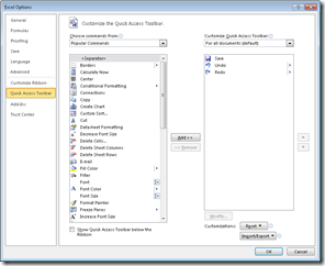
You can add a command to the Quick Access Toolbar simply by right-clicking the command and choosing Add To Quick Access Toolbar. You can also add commands by clicking File in the upper-left portion of the ribbon. Next click Options, and then display the Customize the Quick Access Toolbar page (shown in the second screen shot below).
After choosing a command you want to add, select Add, and click OK. Of course, the Move Up and Move Down arrows let you customize the order in which icons appear. You can remove any command from the Quick Access Toolbar by right-clicking the command, and then clicking Remove From Quick Access Toolbar. You can move the Quick Access Toolbar below the ribbon by right-clicking the toolbar, and selecting Show Below The Ribbon.
Screen Shot: You can add, remove, and arrange commands on the Quick Access Toolbar.
People sometimes have trouble finding commands that appeared in earlier versions of Excel but seem to have disappeared from Excel 2010.
For example, you might be a fan of the old method used to create PivotTables: the layout method. If you still want to use the layout method, you can find it by clicking the drop-down arrow to the right of Popular Commands and choosing Commands Not In The Ribbon. After scrolling down (pressing the P key several times is probably quicker!), you will find the PivotTable And PivotChart Wizard command, which you can then add to your Quick Access Toolbar.
